Continuous Probability Less Than Vs Less Than or Equal to

In today's post, I'm going to give you intuition about the Bernoulli distribution. This is one of the simplest and yet most famous discrete probability distributions. Not only that, it is the basis of many other more complex distributions.

This post is part of my series on discrete probability distributions.

In my introductory post on probability distributions I gave you some intuition about the two main types: discrete and continuous. And in a follow-up post, I showed you the general formulas for calculating the mean and variance of any probability distribution.

The goal of this post is to give you more details and intuition about the most famous of all discrete probability distributions, including its probability mass function, mean, and variance.

• Introduction
  • History of the Bernoulli distribution
• The Bernoulli distribution
  • Parameters and probability mass function
  • The mean of a Bernoulli distribution
  • The variance of a Bernoulli distribution
• Bernoulli distribution plots
• Summary

Introduction

In the overview post on discrete probability distributions, I showed you that you can see the main distinction between discrete and continuous probability distributions in the sample spaces associated with them.

In short, the sample space of a discrete probability distribution is either finite or countably infinite. On the other hand, the sample space of a continuous probability distribution is uncountably infinite. Therefore, you can think of discrete sample spaces as subsets of natural numbers and of continuous sample spaces as subsets of real numbers. You can read more about this in the section discussion discrete sample spaces.

I also told you that every discrete probability distribution is actually a class of specific distributions defined by a probability mass function (PMF). The specific distributions are associated with specific values of one or more parameters of the PMF. You can read more about this in the parameters section of the same post.

The Bernoulli distribution deals with random variables that have exactly 2 possible outcomes. And it simply assigns a probability to each of those outcomes. Pretty simply, isn't it?

A single realization of a Bernoulli random variable is called a Bernoulli trial. On the other hand, a sequence of realizations is called a Bernoulli sequence or, more formally, a Bernoulli process. Different types of Bernoulli sequences give rise to more complicated distributions, like the binomial distribution and the Poisson distribution.

Before I show you the details of the Bernoulli distribution, let me tell you a few words about its name.

History of the Bernoulli distribution

Jacob Bernoulli

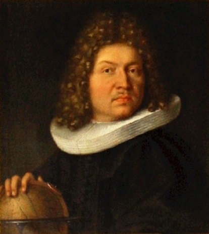
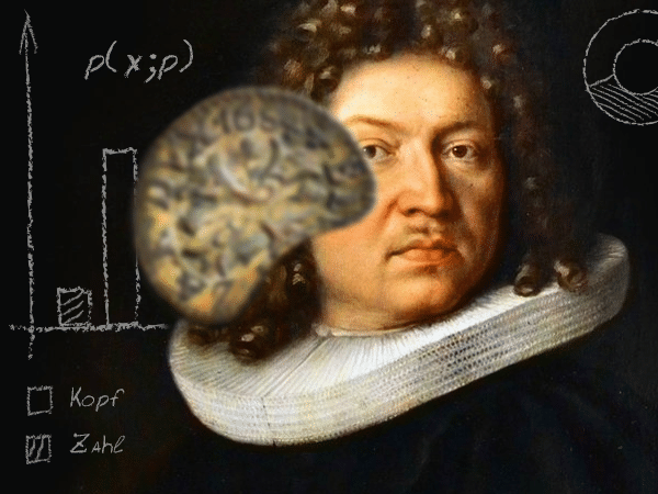
The name of this distribution and all related terms comes from the 17th century Swiss mathematician Jacob Bernoulli. Now, he wasn't really the one who coin the term itself. At the time the concept of a probability distribution hadn't even been discovered yet.

The distribution is named after Bernoulli because he was the one who explicitly defined what we today call a Bernoulli trial. Namely, an experiment with only two possible outcomes. For convenience, these outcomes are usually called "success" and "failure" (but don't read too much into these labels). This tradition started from Bernoulli himself in his book Ars Conjectandi ("The Art of Conjecturing"), published 8 years after his death. Take a look at this quote:

To avoid tedious circumlocution, I will call the cases in which a certain event can happen fecund or fertile. I will call sterile those cases in which the event can not happen. I will also call experiments fecund or fertile in which one of the fertile cases is discovered to occur; and I will call nonfecund or sterile those in which one of the sterile cases is observed to happen.

Many historians consider Ars Conjectandi the founding document of mathematical probability. It presents the first formal solutions to challenging probability problems and introduces fundamental concepts from combinatorics, like permutations and combinations (if curious about those, check out my post on combinatorics).

The above quote is from another remarkable part of the book in which Bernoulli presents the first proof of what we today call the law of large numbers (LLN). He proved the weak version of the law by analyzing the behavior of hypothetical infinite sequences of "success"/"failure" trials with a fixed probability. For more information, check out my post on the LLN.

The Bernoulli distribution

Let's consider some examples of real-world processes that can be represented by a Bernoulli distribution. We're looking for random variables with only 2 possible outcomes. In other words, we want random variables whose sample space has exactly 2 elements.

Well, you can actually take any process and divide its sample space into 2 parts by any well-defined criterion. Let's consider a few processes:

• Flipping a coin
• Rolling a 6-sided die
• Drawing a random card from a 52-card deck
• Spinning a roulette wheel

Coin flipping has a natural Bernoulli distribution if you are considering the probability of "heads" or "tails". Rolling a die could be accommodated if you divide the 6 possible outcomes in 2 groups, like "odd vs. even" or "1/5 vs. 2/3/4/6". With the card drawing example, you could also divide the 52 possible outcomes into 2 groups, like "red vs. black suit". Similarly, with a roulette wheel, you could divide the outcomes into, say, "less than vs. greater than or equal to 10".

All these are examples of repeatable physical processes. However, the Bernoulli distribution is more general and you can apply it for calculating Bayesian or even logical probabilities (see my post on interpretations of probabilities). These can be probabilities of hypotheses or statements (present, past, and future). For example, probabilities coming from questions like "did it rain yesterday?", "is it currently raining?", and "will it rain tomorrow?" can also be represented by a Bernoulli distribution.

Bottom line is, anytime you're dealing with a sample space that consists of only 2 outcomes, you're dealing with a Bernoulli distribution.

Parameters and probability mass function

In the overview of discrete distributions post, I showed you a general notation for the PMF of any distribution:

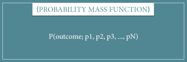
Intuitively, you can read this as "the probability of the outcome, given the parameters of the function".

The Bernoulli distribution has a single parameter, often called p. The value of p is a real number in the interval [0, 1] and stands for the probability of one of the outcomes.

Here's what the probability mass function of a Bernoulli distribution looks like:

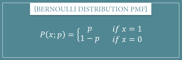
Here x stands for the outcome. A simple way to read this is:

• The probability of the outcome 1 is p
• The probability of the outcome 0 is (1 – p)

If you put any other value for x (besides 0 or 1), the distribution will return a probability of 0.

For example, in coin flipping p stands for the bias of the coin. And in the card drawing example, p stands for the the proportion of red/black suits in the deck. Notice that:

So, it really doesn't matter which outcome's probability you choose to represent with p, as long as you're consistent.

By the way, if you want to see a simple example of Bayesian parameter estimation for Bernoulli distributions, check out my post on estimating a coin's bias.

The mean of a Bernoulli distribution

Remember the general formula for the mean of a discrete probability distribution:

In words, it's equal to the sum of the products of all outcomes and their respective probabilities. Well, the Bernoulli distribution has only 2 parameters, so we can easily calculate its mean:

Pretty simple. What the means, of course, is that the average of a sequence of Bernoulli trials is going to be approaching p, as the number of trials approaches infinity. As Bernoulli himself proved!

And as I showed you in the post on the law of large numbers. Let me borrow an example from that post where I wrote a short simulation of 1000 random flips of a fair coin (p = 0.5):

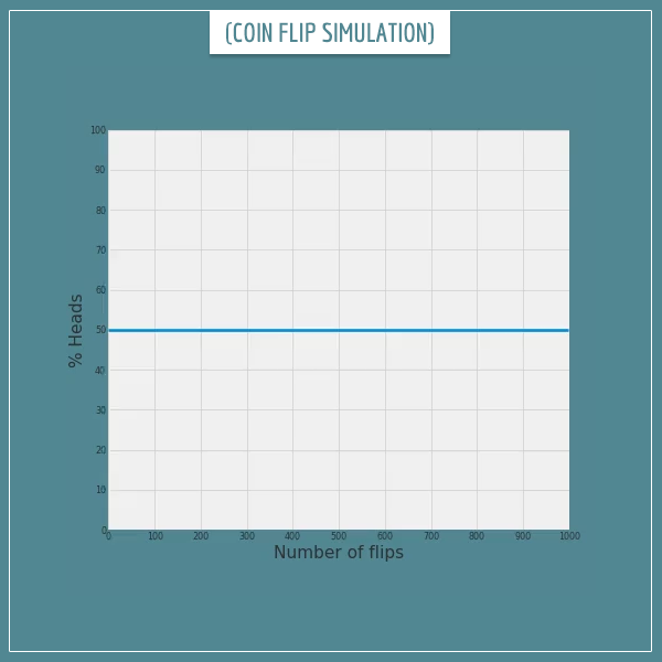
Click on the image to start/restart the animation.

You see how the percentage of "heads" outcomes fluctuates around the expected percentage of 50 and gradually converges to it. If the number of flips were much larger (like 1 million), the % Heads would be almost exactly 50% (or 0.5).

The variance of a Bernoulli distribution

Now let's remember the general formula for the variance of a discrete probability distribution:

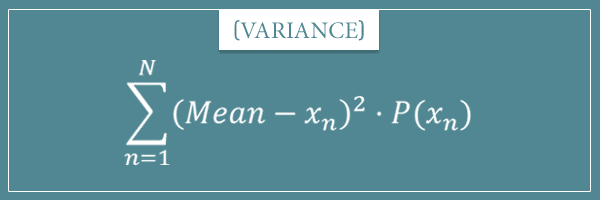
To calculate the variance, we first need to have calculated the mean of the distribution. Which we did. For a Bernoulli distribution it's equal to the parameter p itself. Therefore:

Now let's simplify:

Both forms in the last line are simple enough but the convention is to use the second. Therefore, the variance of a Bernoulli distribution is:

Notice that this is simply multiplying the probabilities of the two possible outcomes. So, the mean of a Bernoulli distribution is the probability of one of the outcomes and the variance is the product of the probabilities of the two outcomes. There's some beauty in this simplicity, isn't there?

Also, notice that the variance is equal to zero when p = 0 or p = 1. This is because each of those values for p implies complete certainty of the outcomes (either all 0s or all 1s). Which essentially makes it a deterministic variable with no variance. Take a look at a plot that shows the variance of a Bernoulli distribution as a function of the parameter p:

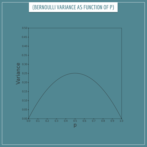
Notice how the variance has a maximum value of 0.25 when p = 0.5 and gradually reduces to 0 as p goes further away from 0.5. Intuitively, this is so because the closer p is to 0.5, the more diverse a sequence of outcomes will be (and vice versa).

Bernoulli distribution plots

Now, to get more intuition about the Bernoulli distribution, let's take a look at a few plots with different values for the parameter p. Like I said, the Bernoulli distribution is a class of infinitely many specific distributions for each possible value of p.

This is what a Bernoulli distribution with p = 0.5 looks like:

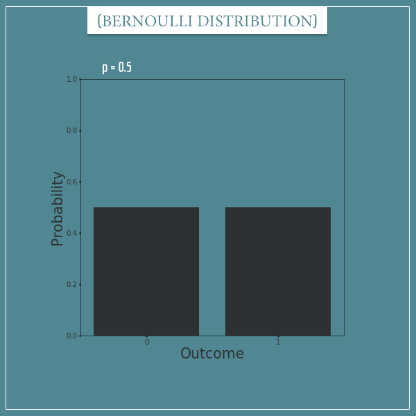
This is also the distribution of flipping a fair coin or any other random variable with 2 equally likely outcomes.

Here's a plot of the distribution with p = 0.3:

This distribution could represent things like flipping a biased coin, drawing a red ball from a pool of 30% red and 70% green balls, and so on.

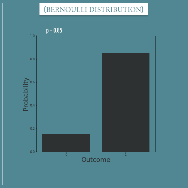
And here's what the distribution looks like with p = 0.85:

Let's finally take a look at an animation that shows the full class of Bernoulli distributions, as p goes from 0 to 1:

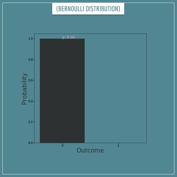
Click on the image to start/restart the animation.

Yep, you just saw (a sparse subset of) the full range of Bernoulli distributions that have ever existed and will ever exist!

Summary

In today's post I introduced one of the simplest probability distributions. The Bernoulli distribution is named after the Swiss mathematician Jacob Bernoulli. It is a discrete probability distribution that represents random variables with exactly two possible outcomes. The probabilities can be related to repeatable physical processes, as well as the truth of past, present, or future hypotheses.

The Bernoulli distribution has a single parameter, p, which defines a very simple probability mass function — p for one of the outcomes and (1 – p) for the other outcome:

From the PMF, using the general mean and variance formulas for discrete probability distributions, we derived equally simple formulas:

Well, that's it for today. I hope you found this post useful. Stay tuned for my future posts from my series on probability distributions!

highsmithhicave.blogspot.com

Source: https://www.probabilisticworld.com/bernoulli-distribution-intuitive-understanding/

Share this post